Choosing A Modelling Method
Introduction
In order to fit a species distribution model (SDM), we must select a modelling method to relate our response data (e.g., presence-background points) to our covariates (e.g., mean annual temperature). There are multiple modelling method available, so how do we select the one appropriate for our analysis?
With an abundance of SDM methods available, it can be difficult to know which to choose. Primarily, the modelling method we choose depends on the type of data we want to analyse and the question we want to ask. Methods for species distribution modelling fall into three broad categories: ‘profile’, ‘regression’, or ‘machine learning’. There are also ensemble models that combine analyses from multiple methods into a single result. Here we confine our discussion to regression and machine learning-based methods. The literature refers to the models under these headings, and we keep to convention, but note that there is no fundamental distinction between the two.
This guide goes into detail about some common modelling methods currently available as modules in zoon. For each method we will cover compatible data types, the underlying statistical approach, and demonstrate how to fit them in zoon.
Throughout these examples we will use presence-only data for the Carolina wren, Thryothorus ludovicianus, in North America, and generate 1000 background points. Figure 1 below is a visualisation of our data.
ext <- extent(c(-138.71, -52.58, 18.15, 54.95)) # define extent of study area

data <- workflow(occurrence = SpOcc("Thryothorus ludovicianus",
                                    extent = ext),
                 covariate = Bioclim(extent = ext),
                 process = Background(1000),
                 model = NullModel,
                 output = PrintOccurrenceMap,
                 forceReproducible = TRUE)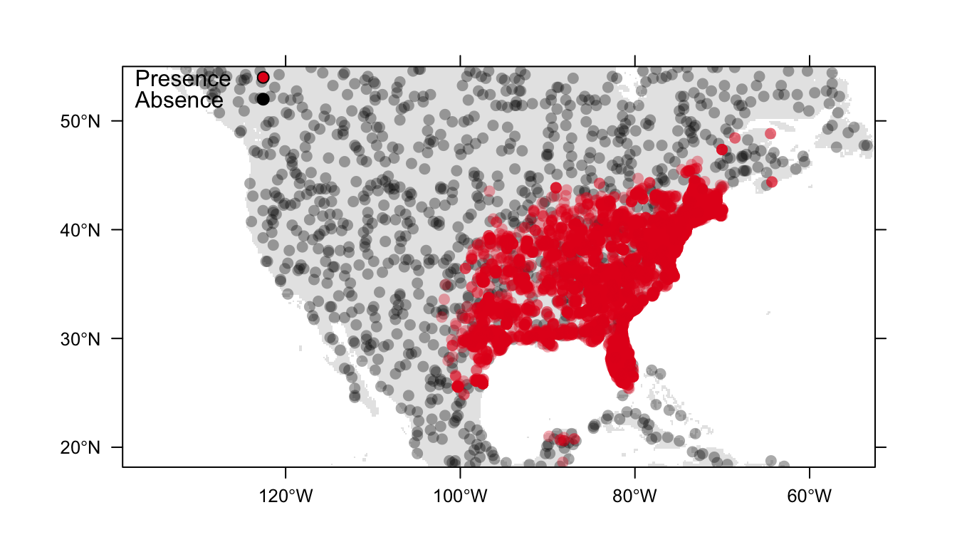
Figure 1: Distribution of presence (red) and background (black) data for the Carolina wren in North America
Regression-based methods
Regression analyses estimate the statistical relationship between a dependent variable (e.g. presence of a species) and one or more independent variables (e.g. environmental covariates). There are currently two regression-based SDMs available as zoon modules: logistic regression and generalised additive models.
Standard linear models assume a linear effect of covariates ,\(x\), on the response variable ,\(y\) (see \((1)\)). These models assume the response variable varies linearly with the covariates, and rely on normally-distributed response variables. In contrast, generalised linear models (GLMs) make use of ‘link functions’ to allow us to relax the assumption of linearity. They let us use non-normally distributed response variables (such as binary data) by transforming them to be used within the standard linear model framework.
\[y = c + mx (1)\]
Logistic regression
Logistic regression is onesuch generalised linear model (GLM) that can be fit to presence/background or presence/absence data. It uses the logit link function to estimate the probability of a binary response variable (e.g. species presence/absence) based on its relationship with our predictor covariates. Logistic regression estimates one regression coefficient (\(\beta\) in the \((2)\)) for each covariate using maximum likelihood estimation. We also estimate an \(Intercept\) term (\(c\) in \((1)\)) like in a standard linear model.
\[logit(Pr(Occurrence)) = Intercept + \beta_1Covariate_1 + \beta_2Covariate_2 + \beta_3Covariate_3 (2)\]
The left-hand side of equation \((2)\) is the transformation of the response variable using the link function. The right-hand side of this equation is known as the linear predictor.
In zoon, we can estimate a species distribution using a logistic regression model by choosing the LogisticRegression model module in our zoon workflow. LogisticRegression uses the glm package.
logistic <- workflow(occurrence = SpOcc("Thryothorus ludovicianus",
                                        extent = ext),
                     covariate = Bioclim(extent = ext),
                     process = Background(1000),
                     model = LogisticRegression,
                     output = PrintMap)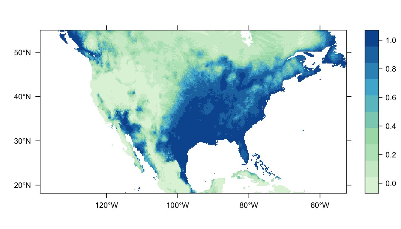
Figure 2: Predicted Carolina wren distribution map from the logistic regression SDM.
In Figure 2 above you can see that the logistic regression model predicts a high probability of occurrence in the eastern USA which broadly matches the distribution of our presence points. There are also patches of high probability of occurrence in western USA, and these likely represent areas of suitable habitat for the Carolina wren that it does not have the dispersal ability to reach.
Generalised additive model
Generalised additive models (GAMs) are similar to GLMs but allow more flexibility. Fitting a GAM for binary data (presence-background or presence-absence) is done using a logit link function. The use of different link functions allows us to use different types of data. The main difference between GAMs and GLMs is that GAMs do not estimate regression coefficients. Instead, the linear predictor is the sum of a set of smoothing functions (see \((3)\) below). Smoothing functions let us fit complex, non-linear relationships between our dependent and independent covariates. Since there are no paramters to estimate in the model GAMs are non-parametric models. Thus the estimated shape of the smoothing function for a covariate is dependent on the data and not set by model parameters (such as defining a quadratic term in a GLM).
\[logit(Pr(Occurrence)) = Intercept + f_1(Covariate_1) + f_2(Covariate_2) + f_3(Covariate_3) (3)\]
When we use smoothing functions without any restrictions, however, it is possible to overfit the model to our data. Models that are overfit pick up on the random error (or noise) in the dataset instead of the underlying relationships with covariates. This means they have poor predictive ability since they overreact to minor variations in the training data. To avoid this GAMs use penalised likelihood maximisation which penalises the model for each additional smoothing function (or ‘wiggliness’).
In zoon, the mgcv model module fits a GAM using the mgcv package. To fit a GAM we need to define a couple of parameters that determine how wiggly and complex the linear predictor can be. Specifically, we need to define the maximum degrees of freedom, \(k\), and the penalised smoothing basis, \(bs\). Together these two parameters balance the model’s representation of the data with the risk of overfitting the model to the dataset. You can find more details on selecting these parameters using ?mgcv::choose.k and ?mgcv::smooth.terms.
Let’s just start by fitting a GAM (using the default settings of \(k\) and \(bs\)) in our workflow.
GAM <- workflow(occurrence = SpOcc("Thryothorus ludovicianus",
                                   extent = c(-138.71, -52.58, 18.15, 54.95)),
                covariate = Bioclim(extent = c(-138.71, -52.58, 18.15, 54.95)),
                process = Chain(StandardiseCov,
                                Background(1000)),
                model = mgcv(k = -1,
                             bs = "tp"),
                output = PrintMap)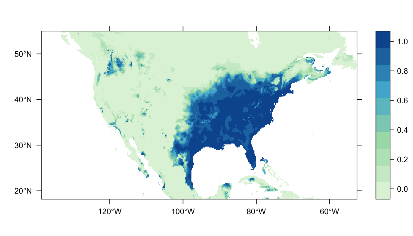
Figure 3: Predicted Carolina wren distribution map for the GAM SDM
Figure 3 above shows the predicted distribution of the Carolina wren from the GAM SDM. Like the logistic regression SDM there is a large patch of high probability of occurrence in the eastern USA that broadly matches the locations of our presence records. In contrast to the logistic regression SDM, however, there is markedly lower predicted probabilities of occurrence in the western USA.
Machine learning methods
Machine learning is a field of computer science where modelling algorithms iteratively learn from data without being explicitly programmed where to look for insight. This is in contast to regression models like GLMs and GAMs that belong to a field of mathematics which finds relationshipis between variables.
MaxEnt/MaxNet
MaxEnt is one of the most widely used SDM modelling methods (Elith et al. 2011). MaxEnt is used only for presence-background data. MaxEnt maximum entropy estimation to fit a model to data.
Maximum entropy estimation compares two probaility densities of our data. First, the probability density of our environmental covariates across the landscape where the species is present, \(f_1(z)\). Second, the probability density of the covariates for our background points, \(f(z)\). The estimated ratio of \(f_1(z)/f(z)\) provides insight on which covariates are important, and establishes the relative suitability of sites.
MaxEnt must estimate \(f_1(z)\) such that it is consistent with our occurrence data, but as there are many possible distributions that can accomplish this it chooses the one closest to \(f(z)\). Minimising the difference between the two probability densities is sensible as, without species absence data, we have no information to guide our expectation of species’ preferences for one particular environment over another.
The distance from \(f(z)\) represents the relative entropy of \(f_1(z)\) with respect to \(f(z)\). Minimising the relative entropy is equivalent to maximising the entropy (hence, MaxEnt) of the ratio \(f_1(z)/f(z)\). This model can be described as maximising entropy in geographic space, or minimising entropy in environmental space.
MaxEnt needs to estimate coefficients in a manner that balances the above constraints with the risk of overfitting the model. This is achieved using regularisation, which can be thought of as shrinking the coefficients towards zero by penalising them to balance model fit and complexity. Thus, MaxEnt can be seen as fitting a penalised maximum likelihood model.
The MaxEnt module uses the maxent() function in the dismo package, and requires a MaxEnt installation on our computer. The zoon helper function GetMaxEnt() is available to help with this installation. Due to common difficulties in downloading MaxEnt, in this example we will use MaxNet as a subsitute. The MaxNet module uses the maxnet R package to fit MaxEnt models without requiring the user to install the MaxEnt java executable file. You select this model in your workflow as follows:
MaxNet <- workflow(occurrence = SpOcc("Thryothorus ludovicianus",
                                      extent = ext),
                   covariate = Bioclim(extent = ext),
                   process = Background(1000),
                   model = MaxNet,
                   output = PrintMap)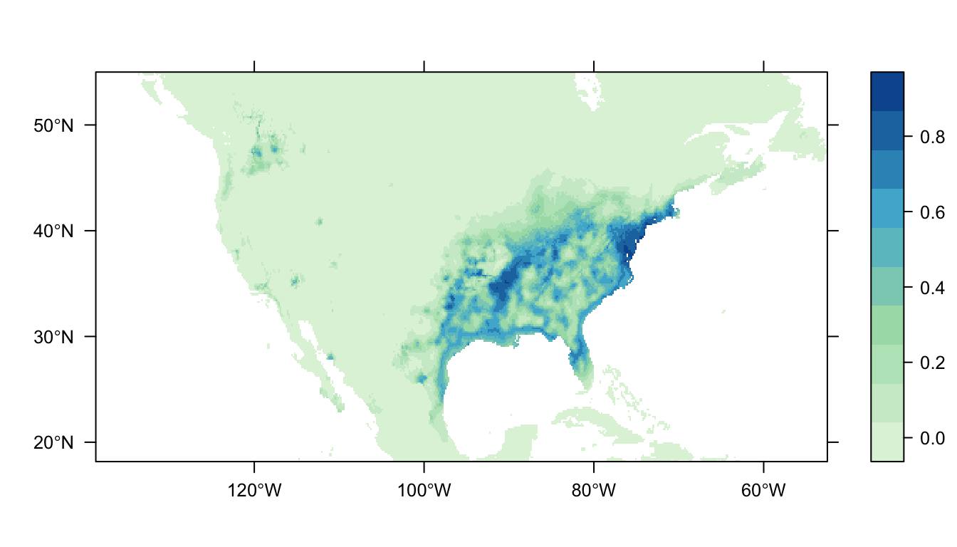
Figure 4: Predicted Carolina wren distribution map for the MaxNet SDM
In Figure 4 above we can see the predicted distribution of the Carolina wren from the MaxNet model. The probability of occurrence within the range of our presence points is markedly smaller than for the GLM- and GAM- based SDMs. There is also a reduced amount of non-zero predictions outside of the range of our presence points (that are also at a lower probability).
RandomForest
Random forest models (RF) are a machine learning technique that produces a single prediction model in the form of an ensemble of weak prediction models (e.g. decision trees). This is in contast to the standard regression approach of fitting a single best model using some information cirterion like AIC.
Decision trees partition the predictor space with binary splits to identify the regions with the most homogenous responses to the predictor variables (see Figure 1 below). A constant value is then fit to each region: either the most probable class for classification models, or the mean response for regression models. The growth of a decision tree involves recursive binary splits, such that binary splits are applied to its own outputs until some criterion is met (such as a maximum tree depth). For example, predictor space could be split at a node for mean annual temperature < or >= 10C, and then the < 10C branch split at mean annual rainfall < or >= 500 mm. The “end” of a branch in a tree thus shows the estimated response variable for a given set of covariates e.g. mean annual temperature >= 10C and mean annual rainfall <500 mm.

*Figure 5: A single decision tree (upper panel), with a response Y, two predictor variables, X1 and X2 and split points t1 , t2 , etc. The bottom panel shows its prediction surface (after Hastie et al. 2001). Image sourced from Elith et al. (2008)
An RF model independently fits multiple decision trees to boot-strapped samples of the data. The final predicted output is the mean prediction of all of the trees. This is to correct for the tendency of decision trees to over-fit their data. Put simply, the core of this idea is that it is easier to build and average multiple rules of thumb than to find a single, highly accurate prediction rule.
The RandomForest module can be fit to presence-background or presence-absence data using the following call in your workflow:
RandomForest <- workflow(occurrence = SpOcc("Thryothorus ludovicianus",
                                            extent = ext),
                         covariate = Bioclim(extent = ext),
                         process = Background(1000),
                         model = RandomForest,
                         output = PrintMap)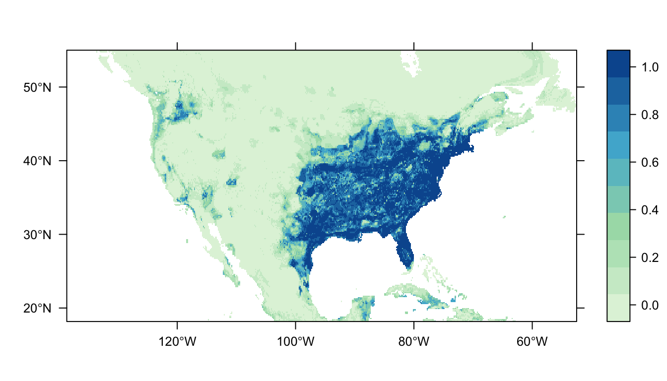
Figure 5: Predicted Carolina wren distribution map for the random forest model.
In Figure 5 above we can see the predicted distribution of the Carolina wren from the RF model. Once again we see an area of high probability of occurrence in the eastern USA matching the range of our presence-records, but the map appears “patchier”. There are also some small predicted patches of occupancy in the western USA (more than GAMs/MaxNet, less than GLM).
Boosted regression trees
Like RF models, Boosted regression trees (BRTs) produce a prediction model in the form of an ensemble of weak prediction models (e.g. decision trees). BRTs are known by various names (including gradient boosting machine, or GBM), but BRT is the name most commonly used in the SDM context.
In contrast to RF models, where each tree is independent, BRTs utilise the boosting technique to combine relatively large numbers of trees in an adaptive manner to optimise predictive performance. This is an iterative procedure that fits each subsequent tree to target the largest amount of unexplained variance from the preceeding trees. This gradually increase the emphasis on observations modelled poorly by existing trees.
The GBM module fits a generalised boosted regression model using the gbm package, and it can be fit to both presence-background and presence-absence datasets. This requires us to set several tuning parameters to control tree and model complexity. The maximum number of trees, max.trees, is equivalent to the number of maximum number of iterations in the model. The maximum depth of each tree, interaction.depth, controls the number of nodes (or splits) allowed in the decision trees. Finally, the learning rate/shrinkage factor of the model, shrinkage, determines the contribution of each tree to the final model average.
This model can be fit using the following call in your workflow (using the default values for the BRT module):
BRT <- workflow(occurrence = SpOcc("Thryothorus ludovicianus",
                                   extent = ext),
                covariate = Bioclim(extent = ext),
                process = Background(1000),
                model = GBM(max.trees = 1000,
                            interaction.depth = 5,
                            shrinkage = 0.001),
                output = PrintMap)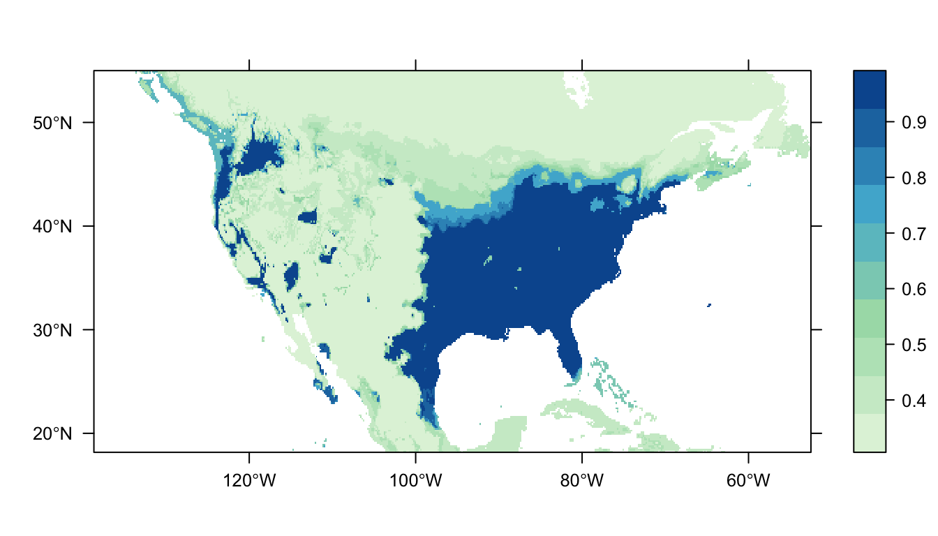
Figure 6: Predicted Carolina wren distribution map for the BRT SDM
In Figure 6 above we can see the predicted distribution of the Carolina wren from the BRT model. Once again we see a large patch of high probability corresponding to the range of our presence points, but also a larger amount of patches in western USA. The overall tendency for predictions to be near 0 or 1 suggests that the model run with the default parameters is overfit to the data.
The XGBoost software is increasingly used in machine learning applications for fitting BRTs to very large datasets. You can use the MachineLearn module to fit BRT models with XGBoost by replacing the model module above with: MachineLearn(method = 'xgbTree').
Choosing a modelling method
The most common SDM modelling methods have been highlighted above, but the question remains about whih method to choose. In short, there are no set rules to determine which method you should use. The way that the methods operate can rule some options out. For example, if you have presence-absence data you wouldn’t use MaxEnt (which only accepts presence-background data), or if you cared about inference more than prediction you would possibly pick a GLM-based method over a decision tree-based one. Even after making some of these decisions you would still have multiple methods to pick from, and while there may a ‘best’ method there is no expert consensus. One option is to try multiple options and determine which one best fits your data, or combine multiple methods as part of an ensemble model. Choice of modelling method or methods is an important aspect of species distribution modelling, and is at least partly dependent on the type of analysis you are trying to perform. This guide has outlined the options available, but ultimately the choice of modelling method is up to you.
Elith, J., Leathwick, J.R. & Hastie, T. (2008). A working guide to boosted regression trees. Journal of Animal Ecology, 77, 802–813.
Elith, J., Phillips, S.J., Hastie, T., Dudík, M., Chee, Y.E. & Yates, C.J. (2011). A statistical explanation of maxent for ecologists. Diversity and Distributions, 17, 43–57.