Data exploration
Introduction
When we undertake a Species Distribution Model (SDM) we use both species occurrence data collected from field surveys or collated observations, as well as environmental predictor data. Before beginning to use covariate data to model occurrence over space, a crucial first step is to familiarise ourselves with the data and its limitations. It is important to do this before modelling the data, as data exploration can result in consequences for the choice of model applied as well as the accurracy of the inference taken from the model. Equally, choice of model a priori may bring a unique set of assumptions that we need to check for in our data. This guide outlines a few suggested steps implemented in both base R as well as using zoon output and process modules for data exploration (Figure 1), but is by no means exhaustive.

Figure 1. Data exploration considerations for occurence and covariate data
Data summary
To begin to familiarise ourselves with the data, it is very useful to examine summary information, including min, mean, and max values for each covariate that you have loaded. Environmental covariate data is subject to error. For example, maybe the maximum value in your elevation variable is 1000 m, but you know that the highest peak in your study region is only 500 m. Maybe your vegetation classification shows ten levels despite it being an eight-category scale.
It can also help us to check the format of the covariates - to ensure continuous variables are stored as numeric data and categorical variables as factors. Categorical variables may be erroneously listed in a numerical index (e.g. vegetation categories identified as 1-10), causing them to be mis-classed. Similarly, if there are any typos in numerical data entries that introduce characters (e.g. ‘2 cm’ instead of ‘2’), then a continuous variable could be classed as a factor.
NA values are to be expected in our raster data as they are commonly masked to cover only a particular region, however finding NA values for covariates in the training data could indicate that some data points have incorrect latitude/longitude values. This can result from being mapped to locations outide the extent of our study, or suggest that the data point sits on the border of the study region and misses the raster due to its resolution and should be adjusted slightly.
With the zoon output module DataSummary, examining covariate data for these potential pitfalls is very easy.
library(zoon)Carolina_Wren_Workflow <- workflow(occurrence = CarolinaWrenPO,
covariate = CarolinaWrenRasters,
process = Background(1000),
model = NullModel,
output = DataSummary)$PointData
longitude latitude pcMix pcDec
Min. :-100.19 Min. :25.10 Min. :-0.28163 Min. :-0.4023
1st Qu.: -90.09 1st Qu.:32.47 1st Qu.:-0.25373 1st Qu.:-0.1441
Median : -84.22 Median :35.90 Median : 0.07983 Median : 1.0642
Mean : -85.09 Mean :35.54 Mean : 0.51684 Mean : 1.4522
3rd Qu.: -80.24 3rd Qu.:38.74 3rd Qu.: 0.81348 3rd Qu.: 2.5997
Max. : -70.01 Max. :43.48 Max. : 9.72729 Max. : 5.7853
pcCon pcGr Lat Lon
Min. :-0.4118 Min. :-0.4333 Min. :-1.47041 Min. :-0.2513
1st Qu.:-0.3641 1st Qu.:-0.4028 1st Qu.:-0.69941 1st Qu.: 0.2841
Median :-0.1350 Median :-0.3277 Median :-0.25919 Median : 0.5832
Mean : 0.2708 Mean :-0.1669 Mean :-0.29397 Mean : 0.5262
3rd Qu.: 0.7252 3rd Qu.:-0.1607 3rd Qu.: 0.09957 3rd Qu.: 0.7851
Max. : 3.5748 Max. : 4.4750 Max. : 0.83779 Max. : 1.1720
$RasterData
pcMix pcDec pcCon pcGr
Min. :-0.28 Min. :-0.40 Min. :-0.41 Min. :-0.43
1st Qu.:-0.28 1st Qu.:-0.40 1st Qu.:-0.41 1st Qu.:-0.38
Median :-0.27 Median :-0.34 Median :-0.27 Median :-0.22
Mean : 0.25 Mean : 0.34 Mean : 0.36 Mean : 0.38
3rd Qu.: 0.06 3rd Qu.: 0.58 3rd Qu.: 0.66 3rd Qu.: 0.55
Max. :10.95 Max. : 5.79 Max. : 5.67 Max. : 5.12
NA's :35451 NA's :35451 NA's :35451 NA's :35451
Lat Lon
Min. :-1.56 Min. :-1.34
1st Qu.:-0.34 1st Qu.:-0.69
Median : 0.22 Median :-0.17
Mean : 0.18 Mean :-0.15
3rd Qu.: 0.74 3rd Qu.: 0.35
Max. : 1.51 Max. : 1.26
NA's :35451 NA's :35451 EXPAND ON WHAT WE SEE ONCE THE UPDATED MODULE PULL REQUEST GOES THROUGH
Outliers/data cleaning
Species distribution datasets are, to varying degrees, reliant on observation records gathered by humans and therefore subject to human error. Even in situations where we are fitting a model to entirely remotely-sensed data such as bioclimatic variables, our species occurrence records are usually pen-and-paper recordings from the field. This manual data entry can lead to mistakes. One way to check for nonsense entries is to the plot occurrence data to covariates one by one, allowing us to isolate unusual entries. For example, if we plotted against latitude, we might see a single occurrence value at a latitude outside the range of our study.
You can visualise these plots using the CovHistogram output module.
Carolina_Wren_Workflow <- workflow(occurrence = CarolinaWrenPO,
                                   covariate = CarolinaWrenRasters,
                                   process = Background(1000),
                                   model = NullModel,
                                   output = CovHistograms)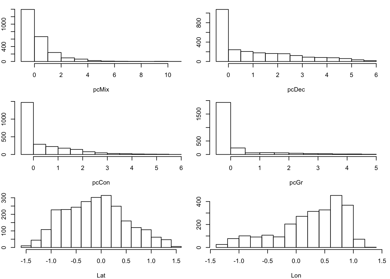
Collinearity
Collinearity is the existence of correlations among covariates, for example between altitude and temperature. For some modelling methods, though notably not all of them, when two covariates in a model are correlated, the modelling method may struggle to identify the impact of each variable independently and the significance of either may be masked. If covariate A and covariate B are correlated, one approach would be to include a single one in the model, preferably based on sound biological justification. Should variable A be included, then in the discussion of the results it will be important to note that the observed effect could equally be driven by correlated covariate B.
You can check for collinearity in many ways, but the simplest is to look at a pair plot of your covariate data. You can do this using the zoon output module PairPlot. The upper panel shows a density scatterplots of relationships between covariates, the diagonal panel shows a density of the points as well as variable names, and the lower panel shows the \(r^2\) correlation values where darker colours indicate stronger correlation (blue in the positive direction, red in the negative).
Carolina_Wren_Workflow <- workflow(occurrence = CarolinaWrenPO,
                                   covariate = CarolinaWrenRasters,
                                   process = Background(1000),
                                   model = NullModel,
                                   output = PairPlot)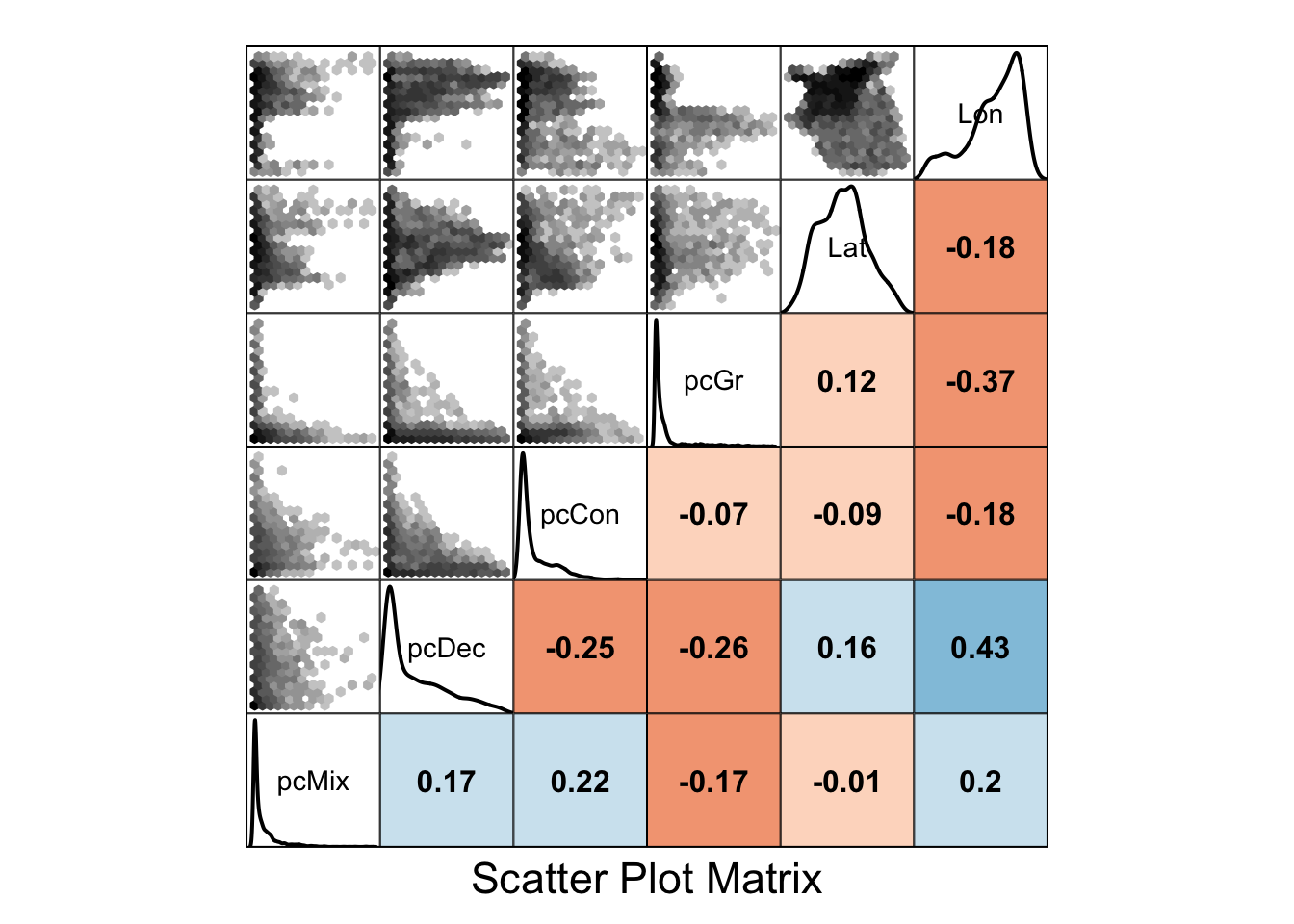
Covariate Report
A tidy summary of many of these data exploration methods is provided with the GenerateCovariateReport Output module. This is based on the GenerateReport() function in the DataExplorer R package, but tailored specifically for SDM analyses. These reports show our data structure, the percentage of missing data, the distribution of our covariates (histograms for continuous data, bar charts for discrete), and show the results of a basic correlation analysis. We need to tell the module which report(s) to generate by setting the type argument to one of “D” (Data Report only), “R” (Raster report only), or “DR” (Data and Raster Report).
output = GenerateCovariateReport(type = "DR")Accessor functions
Where there is no module already designed, we can manipulate our data directly by using the accessor function Process() to generate a dataframe object with extracted raster covariate values for each occurrence point. We can examine the first six rows of this data frame by using the base R function head().
occ.cov.df <- Process(Carolina_Wren_Workflow)$df
head(occ.cov.df)
longitude latitude value type fold pcMix pcDec pcCon
1 -87.50607 34.92022 1 presence 1 0.5902465 1.8175174 -0.2232220
2 -87.78094 34.93984 1 presence 1 0.3973857 1.8771694 -0.1192491
3 -88.05596 34.95882 1 presence 1 1.5005269 2.5864888 0.2768159
4 -86.73598 34.41256 1 presence 1 1.0277690 1.6152677 -0.1380109
5 -86.70923 34.63505 1 presence 1 0.7697110 1.4580649 -0.1153329
6 -86.98288 34.65655 1 presence 1 0.6184651 0.5775564 -0.2159737
pcGr Lat Lon
1 -0.3189337 -0.4050766 0.4139044
2 -0.3031093 -0.4075254 0.3991733
3 -0.2853706 -0.4098892 0.3844383
4 -0.3246833 -0.4765890 0.4622093
5 -0.3219977 -0.4501391 0.4608309
6 -0.3036037 -0.4263944 0.4446908We can check the format of the data with the str() function, or check individual variables with class().
str(occ.cov.df)'data.frame': 2505 obs. of 11 variables:
$ longitude: num -87.5 -87.8 -88.1 -86.7 -86.7 ...
$ latitude : num 34.9 34.9 35 34.4 34.6 ...
$ value : num 1 1 1 1 1 1 1 1 1 1 ...
$ type : chr "presence" "presence" "presence" "presence" ...
$ fold : num 1 1 1 1 1 1 1 1 1 1 ...
$ pcMix : num 0.59 0.397 1.501 1.028 0.77 ...
$ pcDec : num 1.82 1.88 2.59 1.62 1.46 ...
$ pcCon : num -0.223 -0.119 0.277 -0.138 -0.115 ...
$ pcGr : num -0.319 -0.303 -0.285 -0.325 -0.322 ...
$ Lat : num -0.405 -0.408 -0.41 -0.477 -0.45 ...
$ Lon : num 0.414 0.399 0.384 0.462 0.461 ...
- attr(*, "call_path")=List of 1
..$ occurrence: chr "CarolinaWrenPO"
- attr(*, "covCols")= chr "pcMix" "pcDec" "pcCon" "pcGr" ...
- attr(*, "na.action")=Class 'omit' Named int 218
.. ..- attr(*, "names")= chr "218"class(occ.cov.df$pcMix)[1] "numeric"