Data Sources
Introduction
Typically, the first step in species distribution modelling is sourcing species observation records (presence-only, presence-absence, or abundance) and environmental data (such as bioclimatic variables or vegetation maps in the form of rasters) that we will use for our model. In some instances we might be using data we recorded ourselves, other times we might want to use data from public repositories, or even a combination of the two. This tutorial will guide you through the process of accessing some of these data sources within a zoon workflow().
Using the GetModuleList() command we can see all of the Occurrence modules under the $occurrence sub-heading. We can also view the Covariate modules under the $covariate sub-heading.
modules <- GetModuleList()
modules$occurrence [1] "CWBZimbabwe" "CarolinaWrenPO"
[3] "LocalOccurrenceData" "Lorem_ipsum_UK"
[5] "NaiveRandomPresence" "NaiveRandomPresenceAbsence"
[7] "SugarMaple" "UKAnophelesPlumbeus"
[9] "CarolinaWrenPA" "NATrees"
[11] "AnophelesPlumbeus" "SpOcc" modules$covariate[1] "Bioclim_future" "CarolinaWrenRasters" "LocalRaster"
[4] "NaiveRandomRaster" "UKBioclim" "NCEP"
[7] "UKAir" "AirNCEP" "Bioclim"
zoon datasets
zoon comes with several example dataset modules that we can use. These pre-loaded datasets are useful examples for experimenting with zoon modules, or as test datasets when building new modules of your own. For example, SugarMaple provides presence/absence data of sugar maple in North America, CWBZimbabwe provides presence/absence data for the coffee white stem border in Zimbabwe, and NATrees provides occurrence records for 21 eastern North American trees.
To gain familiarity with zoon, we could, for example, choose to fit a model to the Carolina wren data using the CarolinaWrenPO or CarolinaWrenPA occurrence modules (presence-only and presence-absence, respectively) with the CarolinaWrenRasters covariate module.
Carolina_Wren <- workflow(occurrence = CarolinaWrenPO,
covariate = CarolinaWrenRasters,
process = Background(100),
model = NullModel,
output = InteractiveOccurrenceMap)Our own data
SDMs are commonly fit to datasets we have collected ourselves, and zoon has modules to help us load that data. The two modules of interest here are LocalOccurrenceData for our observation records and LocalRaster for our raster-based data. To ensure that all datasets loaded into a zoon workflow() are compatible with model modules, there are specific requirements for the structure and formate of each of these data types, which we will go through below.
The LocalOccurrenceData module requires our data to be saved either as .csv, .xlsx, .tab, or .tsv files and be structured in a very specific format. The first and second columns are the longitude and latitude values (in that order), and the third column is the value of the observation (0 for absence, 1 for presence, or an integer for abundance data). If your coordinate system is not latitude/longitude then you can supply an optional fourth column called CRS that contains the PROJ.4 code for your coordinate system (e.g. +init=epsg:27700 for easting/northing data for the UK). If no CRS column is supplied then latitude/longitude is assumed.
To use the LocalOccurrenceData module you call occurrence in your workflow like this:
occurrence = LocalOccurrenceData(filename = "myData.csv", # File path to your data file
occurrenceType = "presence", # The type of data you have
columns = c(long = "longitude", # The names of the columns in
lat = "latitude", # your .csv that match the
value = "value"), # required columns
externalValidation = FALSE) # Only required if validation
# data is set up externallyRaster data loaded into a workflow using LocalRaster also follows a set format, but it is a simpler process than for occurrence data. This module reads in either a single raster or raster-stack, or a list or vector of rasters and creates a raster-stack. You can find the set of allowed formats for loading rasters by looking at ?writeRasters.
To use this module you call the covariate module like this:
covariate = LocalRaster(rasters = c("myRaster1", # Filepath to a raster
"myRaster2")) # Filepath to a second raster
covariate = LocalRaster(rasters = "myRasterStack") # A RasterStack object already loadedTo serve as an example of loading our own data, here we make use of data on the brown-throated sloth, Bradypus variegatus, provided in the dismo R package. The code below will access this dataset and then do the necessary pre-processing to get it into the correct format.
filename <- paste(system.file(package = "dismo"),
'/ex/bradypus.csv', sep='') # filepath to .csv
Bradypus <- read.csv(filename, header = TRUE) # read in .csv file
Bradypus <- Bradypus[,2:3] # remove columns of species name
Bradypus <- cbind(Bradypus, rep(1, nrow(Bradypus))) # all records are presences, so add column of 1s
colnames(Bradypus) <- c("longitude", "latitude", "value") # set necessary column names
write.csv(Bradypus, "Bradypus.csv") # create a .csv file of the required formatThe raster data available through dismo is in the correct format, but still needs to be loaded into our environment for use.
files <- list.files(path = paste(system.file(package = "dismo"), '/ex', sep=''),
pattern = 'grd', full.names = TRUE ) # list all .grd files in `dismo`
predictors <- stack(files) # create a raster-stack
predictors <- dropLayer(x = predictors, i = 9) # drop unwanted raster layerNow that we have our data in the required format (a .csv file and a raster-stack object) we can fit a model using the LocalOccurrenceData and LocalRaster modules.
Our_Data <- workflow(occurrence = LocalOccurrenceData(filename = "Bradypus.csv",
occurrenceType = "presence",
columns = c(long = "longitude",
lat = "latitude",
value = "value")),
covariate = LocalRaster(predictors),
process = Background(100),
model = NullModel,
output = InteractiveOccurrenceMap)Our output, an interactive occurrence map for the brown-throated sloth, is shown here:
Online repositories
Sometimes we want to source our occurrence and/or covariate data from online sources. Some modules that are useful for sourcing online data include SpOcc, Bioclim, Bioclim-future, and NCEP.
Species occurrence records with SpOcc
The SpOcc module is used to obtain species occurrence records from a selection of online databases, including: GBIF, BISON, iNat, eBird, Ecoengine, and AntWeb. These databases provide free access to species observation records taken by institutions all over the world. This means there is a wealth of data available to ecologists to tackle questions on species distributions without having to undertake costly field work themselves, or to supplement their own observations. The Global Biodiversity Information Facility, or GBIF, is the largest of these repositories (the others restricted by geographical region or taxon). We can call this module like this:
occurrence = SpOcc(species = "SpeciesName", # Species scientific name
extent = c(-1, 0, 51, 52), # Coordinates for the extent of the region
databases = "gbif", # List of data bases to use
type = "presence", # Type of data you want
limit = 10000) # A maximum limit of records to obtainOnline environmental covariate data
The Bioclim module obtains bioclimatic variables from WorldClim. There are 19 bioclimatic variables available that are derived from monthly measurements of temperature and precipitation values to provide more biologically meaningful variables. These variables represent annual trends, seasonality, and limiting factors. This data is available at various resolutions (2.5, 5, or 10 minutes). We can call this module like this:
covariate = Bioclim(extent = c(-180, 180, -90, 90), # Coordinates for the extent of the region
resolution = 10, # Required resolution
layers = 1:5) # Variables we want (between 1-19)We can also obtain these bioclimatic variables for predictions of future climate using the Bioclim_future module. Predicting species distributions under future climate conditions is useful for assessing the effects of climate change on a species for the purposes of conservation. There are multiple models used for predicting climate conditions in the future, and different magnitudes of change, so we must put some thought into the scenario we wish to predict. We can find more information about different scenarios used to predict future climates here and here. Once we have done our research about how type of pathway and model we will use to predict, we can call the Bioclim_future module like this:
covariate = Bioclim_future(extent = c(-10, 10, 45, 65), # Coordinates of the extent of the region
resolution = 10, # Resolution of the data
layers = 1:19, # Required Bioclim variables
rcp = 45, # Representative Concentration Pathways
model = "AC", # General Circulation Models
year = 70) # Time period for the predictionThe NCEP module obtains environmental data from the National Centers for Environmental Prediction. This repository provides a source of environmental variable not available through other repositories, such as air pressure, humidity measures, and soil moisture. For a full list of variables look at ?NCEP.gather. We can call this module like this:
covariate = NCEP(extent = c(-5, 5, 50, 60), # Coordinates of the extent of the region
variables = "hgt", # Character vector of variables of interest
status.bar = FALSE) # Show a status bar of download progress?For example, here we obtain presence-only data for the brown bear, Ursus arctos, in North America from GBIF, and bioclimatic variables from Wordclim.
Online <- workflow(occurrence = SpOcc(species = "Ursus arctos",
extent = c(-175, -65, 20, 75),
databases = "gbif",
type = "presence"),
covariate = Bioclim(extent = c(-175, -65, 20, 75),
resolution = 10,
layers = 1:19),
process = Background(1000),
model = NullModel,
output = InteractiveOccurrenceMap)Data source bias
Now that we’ve seen how to use datasets from different sources, lets construct a workflow using a combination of sources with two sets of occurrence data for comparison. Let’s use CarolinaWrenPO and SpOcc to obtain presence-only data for the Carolina wren and Bioclim for our environmental rasters.
CombinationA <- workflow(occurrence = list(CarolinaWrenPO,
SpOcc("Thryothorus ludovicianus",
extent = c(-138.71, -52.58, 18.15, 54.95))),
covariate = Bioclim(extent = c(-138.71, -52.58, 18.15, 54.95)),
process = Background(100),
model = LogisticRegression,
output = PrintMap)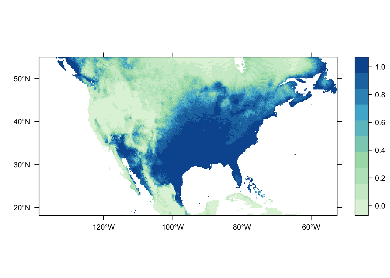
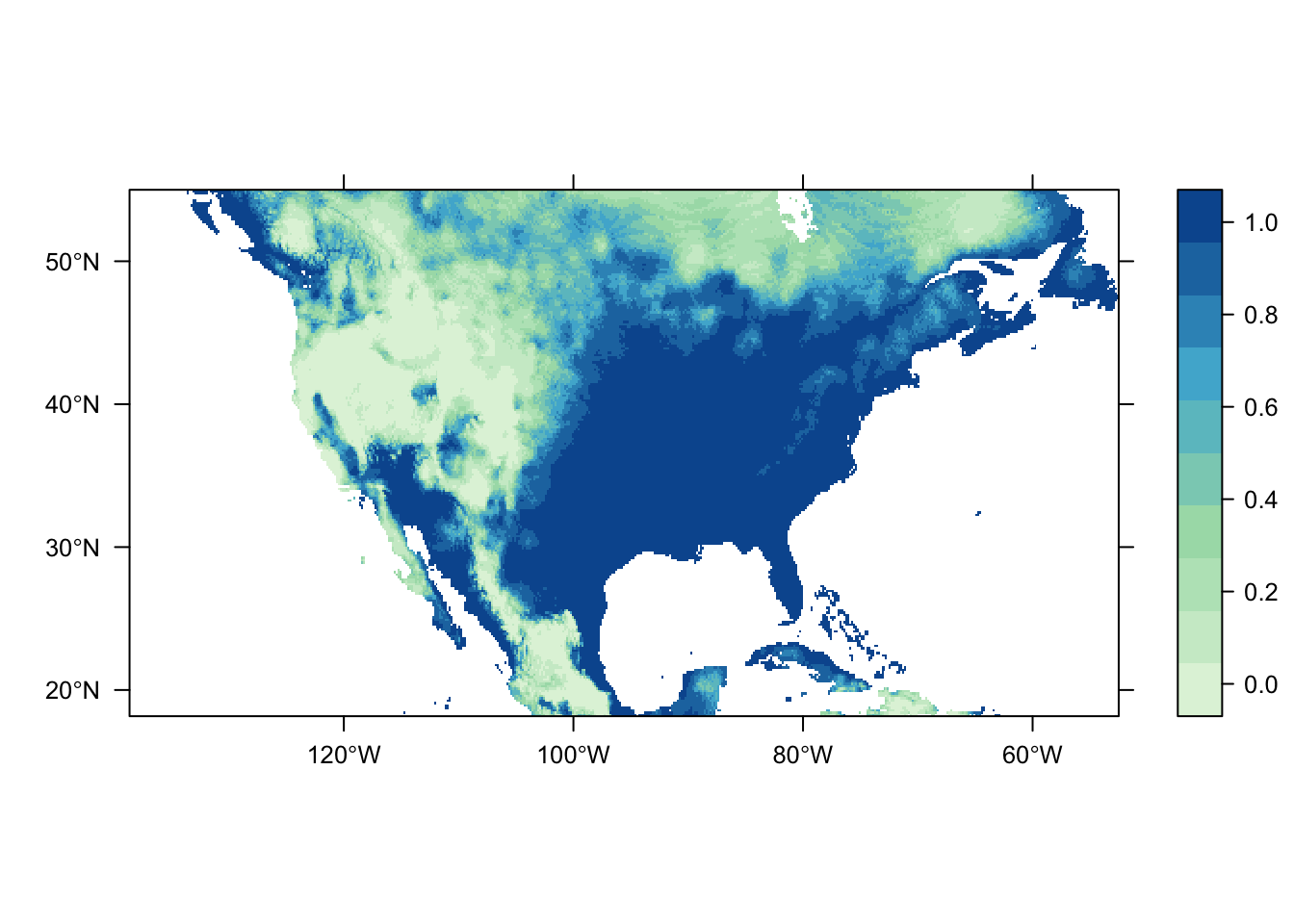
Both of the above plots were generated using the same process and model mdoules; they only differ in the source of their occurrence records. It is obvious that there are significant differences in the predicted distribution of the Carolina wren depending on the dataset chosen. This highlights a very important point to be considered during an analysis: bias in data source. Different data sources are going to have different amounts (and quality) of data-points, and their own inherent sampling biases. Do they contain scientific surveys only? Goverment agency surveys? All occurrence records?
If we pretend that the dataset from CarolinaWrenPO was our own survey data from a study restricted to the contiguous USA, while the SpOcc dataset (via the GBIF repository) includes all occurrence records aross North America (thus including Canada and Mexico), then we have a spatial sampling bias to consider. The latter dataset potentially includes occurrence records outside of the environmental range of the former, which could impact the estimation of the species’ response to the environmental variables.
Other potential sources of bias to consider include the sampled range of environmental variables, spatial sampling bias related to site accessibility (e.g. museum records commonly occur near roads), and reliability of the data source. Source A might have twice the number of occurrence records as Source B, possibly over a larger spatial and/or environmental range, but Source B may be more reliable as it includes records only from trained surveyors to eliminate possibilities of species mis-identification.
Targetted background group
As a final example, lets explore the ability to use the SpOcc module to obtain presence records for species other than our focus species and use them as background data in our model. This can be used to implement a ‘targetted background group’ approach for generating our background data for overcoming observation bias. Here we use presence records of the sedge wren, Cistothorus platensis, and the winter wren, Troglodytes hiemalis, as background data for our Carolina wren analysis. You can see that our background data points are now from geographically similar regions as our presence records rather than randomly distributed throughout the environment.
TargettedBG <- workflow(occurrence = Chain(SpOcc("Thryothorus ludovicianus",
extent = c(-138.71, -52.58, 18.15, 54.95),
type = "presence"),
SpOcc("Cistothorus platensis",
extent = c(-138.71, -52.58, 18.15, 54.95),
type = "background"),
SpOcc("Troglodytes hiemalis",
extent = c(-138.71, -52.58, 18.15, 54.95),
type = "background")),
covariate = Bioclim(extent = c(-138.71, -52.58, 18.15, 54.95)),
process = NoProcess,
model = NullModel,
output = InteractiveOccurrenceMap)