Introduction to SDMs
Why model species distributions?
Knowing where biota are in our world is important for a variety of reasons. We might want to know where an endangered species is most likely to occur so we can protect its habitat, or where a disease will break out so we can prevent it from doing so, or where a species of fish occurs so we can responsibly harvest our fisheries. We can answer all of these questions and more using species distribitions models (SDMs).
Species distribution models predict species distributions by correlating environmental covariates, such as temperature or rainfall, with observations of species occurence - presence, absence, or abundance. While these relationships are correlative, as opposed to mechanistic, they still help us identify potential ecological relationships between species and the environment. This enable us to make ecological inferences.
Environmental response curves, for example, illustrate how the probabilty of species occurrence varies in environmental space, that is, over environmental gradients. Figure 1a shows an example of a response curve for the blue whale, Balaenoptera musculus. This plot shows how blue whale abundance varies along a gradient of sea surface height (SSH) (Redfern et al. 2017).
These species-environment relationships can be used to map the distribution of species in geographic space. Figure 1b shows a predicted distribtion for the Ebola virus (Pigott et al. 2014). Mapping the current distribution of a species can be useful for planning responses to public health emergencies or prioritising habitat conservation, for example.
We can also use SDMs to predict the future distribution of species. For example, we might need to know how changing climate will shift the distribution of a species. By using future climate scenarios to create environmental covariates we can predict the future distribution of species. We could also identify the potential future distribution of an invasive species, in current or future climates. Elith et al. (2010) did just this for the invasive cane toad, Bufo marinus, in Australia. Figure 1c illustrates the current distribution of the cane toad (black line) and the predicted future distribution (grey area).

Figure 1. Species distribution modelling aims: ecological inference (a; figure from Redfern et al. (2017), photo from Cetus.ucsd.edu (2013)), predicting current species distributions (b; figure from Pigott et al. (2014)), or future distributions (c; figure from Elith et al. (2010), photo from Fraser-Smith (2010)).
What are SDMs?
Correlative species distribution models estimate a species’ realised niche. They estimate the probabilty of species occurrence along environmental gradients by correlating occurrence data with environmental covariates. Let’s revisit the ecological theory underlying species distributions.
A species distribution is typically considered the result of three factors: the abiotic environment, the biotic environment, and the species’ dispersal ability (Soberon & Peterson 2005). The intersection of the abiotic and biotic environment constitutes the fundamental niche. This is where the species could potentially occur given what we know of its biology and ecology. However, most species do not occur everywhere they potentially could. Where a species actually occurs is termed the realised niche. For example, a realised niche could be constrained by the climate required for individuals to survive, the local vegetation types it depends on, and its abillity to traverse different landscapes. Species interactions are also considered to constrain the fundamental niche to the realised niche. For example, two closely related species may have mutally exclusive geophraphic distributions despite having similar physiological tolerances, habitat preferences, and dispersal ability.
We have illustrated the SDM fitting process in a flowchart below (Figure 2). We correlated presence data for the Carolina wren in the United States with a suite of environmental covariates, such as the cover of different forest types. We’ve mapped species presence records onto geographic space (Figure 2a; black dots) and a random selection of background points (brown dots), which we used as pseudo-absences in our model. We’ve also plotted these same data in environmental space against two covariates (Figure 2b): percentage of deciduous and mixed forests. By correlating presence-background data with environmental covariates, we’ve predicted the Carolina wren’s probability of occurrence in environmental space (Figure 2c). In the final plot (Figure 2d), we’ve mapped these probabilities back onto geographic space. The Carolina wren is most likely to occur in southeast USA (yellow) and least likely to occur in the northwest (purple). By modelling species distributions, we can begin to understand where species are likely to occur and why.

Figure 2. Species distribution modelling process. Presence-background points in geographic (a) and environmental space (b; P = presence, B = background), and predicted probability of occurrence in environmental (c) and geographic space (d; colour scale represents probability of occurrence).
How can I fit an SDM?
This introductory guide will demonstrate how to use the zoon R package to fit species distribution models. zoon is designed to make fitting SDMs simple and reproducible. zoon keeps things simple by splitting the SDM fitting process into five easy steps:
- Occurence: Gather species occurrence data.
- Covariates: Gather environmental covariates.
- Process: Process data as required.
- Model: Choose a modelling method.
- Output: Produce plots and graphs.
The primary function for fitting SDMs with zoon is workflow(). The workflow() function has five arguments - one for each step in the SDM fitting process. The inputs for each argument are called modules, which determine what data and modelling method we’ll use and what outputs we’ll produce.
Let’s see a zoon workflow in action. Don’t forget to load the package!
library(zoon)A basic workflow for the Carolina wren in the USA could look like this:
workflow <- workflow(occurrence = CarolinaWrenPO,
                     covariate = CarolinaWrenRasters,
                     process = Background(100),
                     model = MaxNet,
                     output = PrintMap)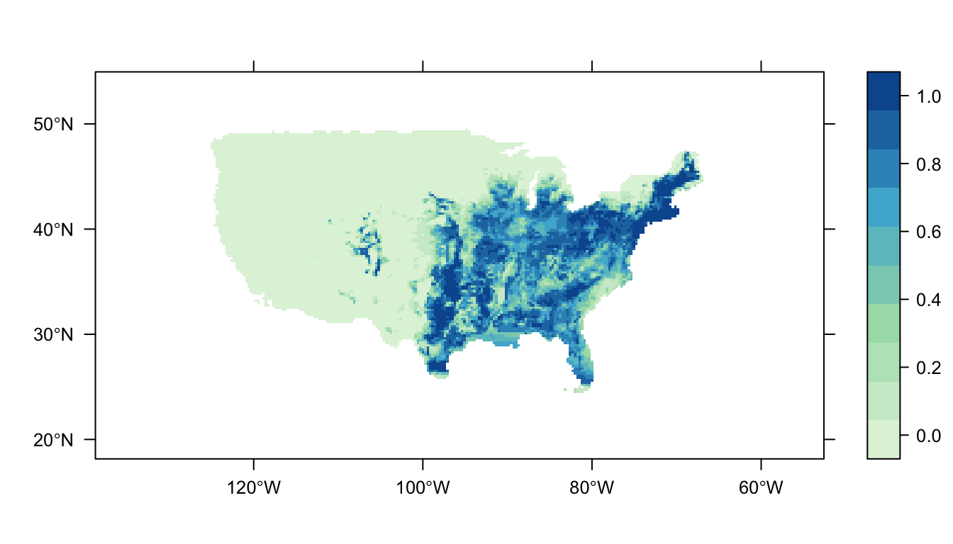
In this workflow, we’ve chosen one module for each argument in workflow(). Using zoon, we’ve:
- Obtained presence-only records for the Carolina wren,
- Loaded the CarolinaWren rasters as environmental covariates,
- Selected 100 background points,
- Fit a MaxNet model and,
- Generated a map as our output.
The printed map illustrates the Carolina wren’s distribution as predicted by our SDM.
We’ll work with this workflow throughout this introductory guide. In order to tackle SDMs one step at a time, we’ll update the arguments one-by-one.
The five steps in zoon
Step 1: Occurrence
The occurrence argument is where we load our species occurrence data. The most common types of species occurrence data are presence-only, presence-background, and presence-absence. Less commonly, SDMs are fit with abundance data.
Presence-only data are usually sourced from museum or herbarium records, or citizen scientists, and consist of a list of observations of a species and the geographic location of the observation.
Presence-background data are the same as presence-only data but they have an associated set of randomly generated ‘background’ points, also called ‘pseudo-absences.’
Presence-absence data generally come from structured field surveys, by novices and experts alike, where the presence or absence of species is recorded for a given location and survey method.
There are three methods for loading data into our workflow. We can use existing occurrence modules in zoon like SugarMaple, we can download data from an online repository using SpOcc, or we can load our own data from a local computer using LocalOccurrenceData. Presence-only data are widely and freely accessible online and as a result are the most commonly used.
zoon has several functions available to view the contents of each module in the workflow. For example, we can view our species occurrence data using the Occurrence() accessor function (using the base R function head() to return only the first six lines):
head(Occurrence(workflow))## longitude latitude value type fold
## 1 -87.50607 34.92022 1 presence 1
## 2 -87.78094 34.93984 1 presence 1
## 3 -88.05596 34.95882 1 presence 1
## 4 -86.73598 34.41256 1 presence 1
## 5 -86.70923 34.63505 1 presence 1
## 6 -86.98288 34.65655 1 presence 1The first and second columns provide the geographic coordinates of the observation as longitude and latitude, the third column is the observation value (1 = presence, 0 = absence), and the fourth column is the type of observation. The fifth and final column identifies the ‘fold’ this data will be fitted in. The function of folds wil be covered in a later zoon guide on model evaluation. The default model has only one fold - all data is fitted simultaneously.
Step 2: Covariates
The covariate argument is where we load our environmental data - our covariate module. As with occurrence modules, there are many different covariate modules to choose from. There are existing modules in zoon that contain data, such as CarolinaWrenRasters, and there are modules that source data from online repositories, such as Bioclim. We could also load our own data from a local computer using LocalRaster.
We can use the Covariate() accessor function to extract our covariates from the workflow. Covariate data in zoon are always rasters and stored as RasterBrick objects.
Covariate(workflow)## class : RasterBrick
## dimensions : 165, 297, 49005, 6 (nrow, ncol, ncell, nlayers)
## resolution : 0.29, 0.223 (x, y)
## extent : -138.7131, -52.58307, 18.1523, 54.9473 (xmin, xmax, ymin, ymax)
## coord. ref. : +init=epsg:4326 +proj=longlat +datum=WGS84 +no_defs +ellps=WGS84 +towgs84=0,0,0
## data source : in memory
## names : pcMix, pcDec, pcCon, pcGr, Lat, Lon
## min values : -0.2816289, -0.4023483, -0.4118219, -0.4333224, -1.5588675, -1.3447938
## max values : 10.949743, 5.785296, 5.671915, 5.118029, 1.505573, 1.255225Using what we’ve learned so far, let’s fit a different SDM by altering our workflow. We’ll build a SDM for the same species, the Carolina wren (Thryothorus ludovicianus), but instead of using pre-exisitng data, we’ll download data from online repositories. To change the occurrence data, we need to change the occurrence module. Instead of CarolinaWrenPO, we’ll download data from online repositories using SpOcc. To change our environmental covariates, we need to change the covariate module. The Bioclim module accesses the Bioclim bioclimatic data.
Both the SpOcc and Bioclim modules require us to specify a geographic extent - this is the boundary of the area we want to retrieve data from. We’ll extract and use the extent from our previous model by saving it to an object called ext. This way, we can compare the two SDMs.
ext <- extent(Covariate(workflow))
ext
## class : Extent
## xmin : -138.7131
## xmax : -52.58307
## ymin : 18.1523
## ymax : 54.9473workflow <- workflow(occurrence = SpOcc("Thryothorus ludovicianus", extent = ext),
covariate = Bioclim(extent = ext),
process = Background(100),
model = MaxNet,
output = PrintMap)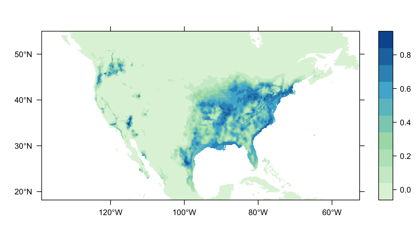
This distribution map is different to our orginal. Given this new set of data, the wren is still most likely to be found in southeast USA. However, now there is a small patch of increased probabilty in the northwest. We have disagreement between two different models! An interesting turn of events.
Try running this workflow for another species!
Step 3. Process
Next it’s time to consider any required data processing. We process our data by choosing modules for the process argument of workflow(). There’s a whole suite of data processing we might want to do before fitting our model. For example, we could clean our data by removing poor data points using the Clean module. The process argument is also where we generate background data points for when we have a presence-only occurrence module. We can actually do both (or more) at once using the Chain() function!
workflow <- workflow(occurrence = SpOcc("Thryothorus ludovicianus", extent = ext),
                          covariate = Bioclim(extent = ext),
                          process = Chain(Clean, Background(100)),
                          model = MaxNet,
                          output = PrintMap)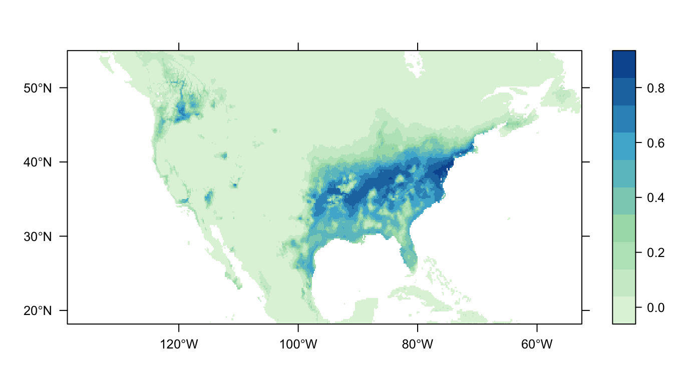
We don’t always need to process our data, in those instances, we can use the NoProcess module.
Step 4. Model
The fourth argument of workflow() is model; this is where we choose our modelling method. There are many modelling methods to choose from and each have their merits (Elith* et al. 2006). To help you choose which model module is right for your data, we’ve written a ‘Choosing A Model’ guide.
For now, let’s work with the common modelling method logistic regression using the module LogisticRegression. We’ll keep our data and process modules the same:
workflow <- workflow(occurrence = SpOcc("Thryothorus ludovicianus", extent = ext),
                     covariate = Bioclim(extent = ext),
                     process = Chain(Clean, Background(100)),
                     model = LogisticRegression,
                     output = PrintMap)
That looks different to our previous MaxNet SDMs, doesn’t it? The areas with higher probabilty of occurrence are much increased!
Step 5. Output
Once we’re happy with our data, modelling method, and data processing, it is finally time to check our results. output is the fifth argument of the zoon workflow function and final step of the zoon SDM fitting process.
Instead of displaying a static map, as we have been so far, let’s use the InteractiveMap module to render an interative map.
workflow <- workflow(occurrence = SpOcc("Thryothorus ludovicianus", extent = ext),
                          covariate = Bioclim(extent = ext),
                          process = Chain(Clean, Background(100)),
                          model = LogisticRegression,
                          output = InteractiveMap())
The InteractiveMap module produces a map of occurrence probability we can interact with. The map has a scale from purple (low probability) to yellow (high probability). By zooming in and around, we can see more closely how our model predictions align with the data. We can also click on our data to get information about it and we can select which data (presence, background, or both) we want to overlay. Have a go!
Now we’ve seen how Carolina wren occurrence varies over geographic space, let’s look more closely at what is driving that variation. How does probability of occurrence vary along the environmental gradients we’ve included in our model? For this, we can use the ResponsePlot module to make graphs of the predicted relationships between probabilty of occurrence and our environmental covariates.
workflow <- workflow(occurrence = SpOcc("Thryothorus ludovicianus", extent = ext),
                     covariate = Bioclim(extent = ext),
                     process = Chain(Clean, Background(100)),
                     model = LogisticRegression,
                     output = ResponsePlot)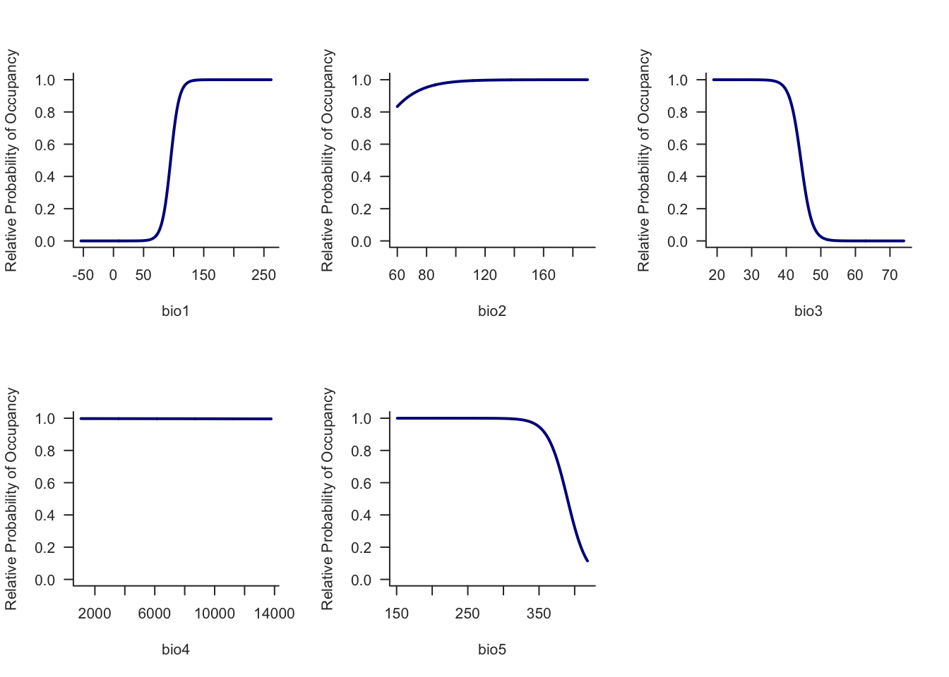
The probability of Carolina wren occurrence increases along the bio1 gradient and decreases with bio3. bio2 appears to have little effect for the Carolina wren.
Saving our work
Our whole analysis and results are stored in the zoon workflow object workflow. This object contains all of the code needed to re-run the analysis, all of the data we used, and all of the results. By saving this object we can always re-load it to access our results, get different outputs, or even try different modelling methods.
We can save workflow as a single .RData object with R’s save() command:
save(workflow, file = 'workflow.RData')and reload it with load():
load('workflow.RData')Because the workflow object contains our whole analysis, we can also share it with collaborators. After they install zoon and load the workflow object, they can access and modify the analysis too.
Conclusion
In this introductory guide, we’ve used zoon to run and interpret a series of species distribution models in a fully reproducible way. First we loaded our occurrence and covariate data for our species of interest. Then we processed that data as required, ran our model, and produced some outputs. Everything needed to reproduce our analysis is stored in our workflow, which we saved and can now share! Why not explore different combinations of modules yourself? Use the GetModuleList() command to get a list of available modules for each of the five zoon steps.
References
Cetus.ucsd.edu. (2013).
Elith*, J., H. Graham*, C., P. Anderson, R., Dudík, M., Ferrier, S., Guisan, A., J. Hijmans, R., Huettmann, F., R. Leathwick, J., Lehmann, A., Li, J., G. Lohmann, L., A. Loiselle, B., Manion, G., Moritz, C., Nakamura, M., Nakazawa, Y., McC. M. Overton, J., Townsend Peterson, A., J. Phillips, S., Richardson, K., Scachetti-Pereira, R., E. Schapire, R., Soberón, J., Williams, S., S. Wisz, M. & E. Zimmermann, N. (2006). Novel methods improve prediction of species’ distributions from occurrence data. Ecography, 29, 129–151.
Elith, J., Kearney, M. & Phillips, S. (2010). The art of modelling range-shifting species. Methods in ecology and evolution, 1, 330–342.
Fraser-Smith, S. (2010). Rhinella marina (linnaeus, 1758) - cane toad.
Pigott, D.M., Golding, N., Mylne, A., Huang, Z., Henry, A.J., Weiss, D.J., Brady, O.J., Kraemer, M.U., Smith, D.L., Moyes, C.L., Bhatt, S., Gething, P.W., Horby, P.W., Bogoch, I.I., Brownstein, J.S., Mekaru, S.R., Tatem, A.J., Khan, K. & Hay, S.I. (2014). Mapping the zoonotic niche of ebola virus disease in africa (P. Jha, Ed.). eLife, 3, e04395.
Redfern, J.V., Moore, T.J., Fiedler, P.C., Vos, A. de, Brownell, R.L., Forney, K.A., Becker, E.A. & Ballance, L.T. (2017). Predicting cetacean distributions in data-poor marine ecosystems. Diversity and Distributions, 23, 394–408.
Soberon, J. & Peterson, A.T. (2005). Interpretation of models of fundamental ecological niches and species’ distributional areas. Biodiversity Informatics, 2.